library(conflicted)
library(tidyverse)
library(httr)
library(brms)
library(ggdist)

conflicts_prefer(dplyr::filter,
                 brms::ar,
                 brms::dstudent_t,
                 brms::pstudent_t,
                 brms::qstudent_t,
                 brms::rstudent_t,
                 stats::lag)

#please use cmdstanr, it's so much faster
options(cores = parallel::detectCores(),
        brms.backend = "cmdstanr",
        pillar.sigfig = 6)

theme_set(theme_minimal())My experience with astronomy and astrophysics boils down to teenage curiosity. The main purpose of this example is as an exercise in
brmsnonlinear syntax. There are probably many tiny errors and things that could be done better. The way the variables are used doesn’t have to reflect the order in which they were inferred, it’s purely a statistical exercise. A more realistic story would be to weigh things on Earth and then use the inferred gravitational constant to find out the mass of astronomical bodies.
What?
In some disciplines, there is a disconnect between scientific theory and use of models and current practice. In physics, for example, theory often results in an explicit functional form, this model is tested against reality, and it is provisionally kept as long as there are no obvious discrepancies with observation. If and when those arise, it’s an incentive to question the model and look for a better one. In many other scientific fields, the role of falsification seems like the opposite: nobody really believes the “null” model represents reality, and observing a lack of fit to data is the goal. Null hypothesis rejected, you discovered something new (maybe) and you win! This contrast has been highlighted several times, for example by Meehl (1967).
It doesn’t have to be like this. Even when fitting statistical models to empirical data, sometimes you’re lucky and theory provides you with a formula that you can use in place of an additive linear model. Chapter 16 of McElreath (2020) is dedicated to examples of this, including one with the Lotka-Volterra equations. Nonlinear model formulas are key to this approach, so, with the purpose of getting in some exercise with them in brms, I have developed the following contrived example:
Let’s fit Kepler’s third law in brms to find the gravitational constant G
What I mean exactly is the formula that you get by substituting Newton’s law of gravitation into Kepler’s law
\[\frac{a^{3}}{T^{2}}=\frac{G(M+m)}{4\pi^{2}}\]
What data to fit this to? I found a website that lets you freely download data about solar system bodies in a machine-readable way. For simplicity, I’m restricting this to moons orbiting around planets, since the two are easy to combine in their data format.
Setup
Get the data
#this is my key, stored locally. You can get your own, it's free
key <- read_lines("apikey.txt")

#moon data
moons <- GET("https://api.le-systeme-solaire.net/rest/bodies/",
           add_headers(Authorization = paste("Bearer", key)),
           query = list(`filter[]` = "bodyType,eq,Moon")) |>
  content()

#planet data
planets <- GET("https://api.le-systeme-solaire.net/rest/bodies/",
               add_headers(Authorization = paste("Bearer", key)),
               query = list(`filter[]` = "bodyType,eq,Planet")) |>
  content()

useful <- c("id", "englishName", "semimajorAxis", "mass", "sideralOrbit", "aroundPlanet")

#wrangle this ugly list into a nice tibble
planets <- planets$bodies |>
  map(\(x) x |>
        #some elements are null, some are lists of length 2
        #as_tibble_row complains, that's why the gymnastics
        discard(is_null) |>
        enframe() |>
        pivot_wider()) |>
  #bind the planet rows into a tibble
  bind_rows() |>
  #keep only what's necessary
  select(any_of(useful)) |>
  #mass is in scientific notation across two fields
  mutate(mass = map_dbl(mass, \(x) x$massValue * 10^x$massExponent)) |>
  #undo the list-cols created by enframe() |> pivot_wider()
  mutate(across(everything(), unlist))

#same as above, but for moons
moons <- moons$bodies |>
  map(\(x) x |>
        discard(is_null) |>
        enframe() |>
        pivot_wider()) |>
  bind_rows() |>
  select(id, englishName, semimajorAxis, mass, sideralOrbit, aroundPlanet) |>
  #some moons have missing mass
  drop_na() |>
  mutate(mass = map_dbl(mass, \(x) x$massValue * 10^x$massExponent),
         #just need the id of the planet
         aroundPlanet = map(aroundPlanet, 1)) |>
  mutate(across(everything(), unlist)) |>
  #there are some bogus entries
  filter(sideralOrbit > 0)

#join planets to moons
data <- moons |>
  inner_join(planets |> select(id, mass),
             by = join_by(aroundPlanet == id),
             suffix = c("_s", "_p")) |>
  mutate(
    #only the sum of masses is identified in the equation
    M = mass_s + mass_p,
    #convert semi-major axis to meters
    a = semimajorAxis * 1000,
    #convert sideral orbit to seconds
    #assuming these are conventional days, not sideral seems to be the right call
    T = sideralOrbit * 24 * 3600,
    #remind the value of pi to the model
    pi = pi)

head(data)| id | englishName | semimajorAxis | mass_s | sideralOrbit | aroundPlanet | mass_p | M | a | T | pi |
|---|---|---|---|---|---|---|---|---|---|---|
| lune | Moon | 384400 | 7.3460e+22 | 27.32170 | terre | 5.97237e+24 | 6.045830e+24 | 384400000 | 2360594.88 | 3.141593 |
| phobos | Phobos | 9378 | 1.0600e+16 | 0.31891 | mars | 6.41712e+23 | 6.417120e+23 | 9378000 | 27553.82 | 3.141593 |
| deimos | Deimos | 23459 | 1.4762e+15 | 1.26244 | mars | 6.41712e+23 | 6.417120e+23 | 23459000 | 109074.82 | 3.141593 |
| io | Io | 421800 | 8.9320e+22 | 1.76914 | jupiter | 1.89819e+27 | 1.898279e+27 | 421800000 | 152853.70 | 3.141593 |
| europe | Europa | 671100 | 4.8000e+22 | 3.55118 | jupiter | 1.89819e+27 | 1.898238e+27 | 671100000 | 306821.95 | 3.141593 |
| ganymede | Ganymede | 1070400 | 1.4819e+23 | 7.15455 | jupiter | 1.89819e+27 | 1.898338e+27 | 1070400000 | 618153.12 | 3.141593 |
Fit the model
Since the data is literally on astronomical scales, I thought it wise to fit the model on a log10-transformed version of the equation. While this might take some of the nonlinear charm away, since a big product is transformed in a more familiar sum, we will see that the nonlinear formula will still let us specify the model in a way that would just break with a traditional model formula.
The parameter to fit is G, but we still need some meaningful outcome on the LHS. I decided to solve for \(\widehat{M} = M +m\)
\[\widehat{M}=\frac{4\pi^{2}a^{3}}{T^2G}\]
Then, taking the log10 of both sides
\[\log M = -\log G+\log4\pi^2+3\log a-2\log T\]
This translates directly into the nonlinear formula. Unlike the usual model formulas, regression coefficients (what you multiply the sum terms with) are explicit, so any parameter must be specified with a unique name in the formula. This lets us say explicitly that the last two terms must be multiplied by 3 and 2, not with parameters estimated from the data. The parameter to estimate, logG, has its own intercept-only model.
formula <- bf(log10(M) ~ -logG + log10(4*pi^2) + 3*log10(a) - 2*log10(T),
              logG ~ 1,
              nl = T)
Since I’m not an astronomer, I’ll pretend I have no domain knowledge outside “planets are big, and moons as well” and use default priors just this once. The model fits fine in case you’re worried.
get_prior(formula, data)| prior | class | coef | group | resp | dpar | nlpar | lb | ub | tag | source |
|---|---|---|---|---|---|---|---|---|---|---|
| student_t(3, 0, 2.5) | sigma | 0 | default | |||||||
| b | logG | default | ||||||||
| b | Intercept | logG | default |
Time to actually fit the model.
fit <- brm(formula, data, seed = 950, silent = 2)

fit
Family: gaussian
Links: mu = identity
Formula: log10(M) ~ -logG + log10(4 * pi^2) + 3 * log10(a) - 2 * log10(T)
logG ~ 1
Data: data (Number of observations: 161)
Draws: 4 chains, each with iter = 2000; warmup = 1000; thin = 1;
total post-warmup draws = 4000
Regression Coefficients:
Estimate Est.Error l-95% CI u-95% CI Rhat Bulk_ESS Tail_ESS
logG_Intercept -10.18 0.00 -10.18 -10.17 1.00 4166 2866
Further Distributional Parameters:
Estimate Est.Error l-95% CI u-95% CI Rhat Bulk_ESS Tail_ESS
sigma 0.03 0.00 0.02 0.03 1.00 1447 1820
Draws were sampled using sample(hmc). For each parameter, Bulk_ESS
and Tail_ESS are effective sample size measures, and Rhat is the potential
scale reduction factor on split chains (at convergence, Rhat = 1).pp_check(fit)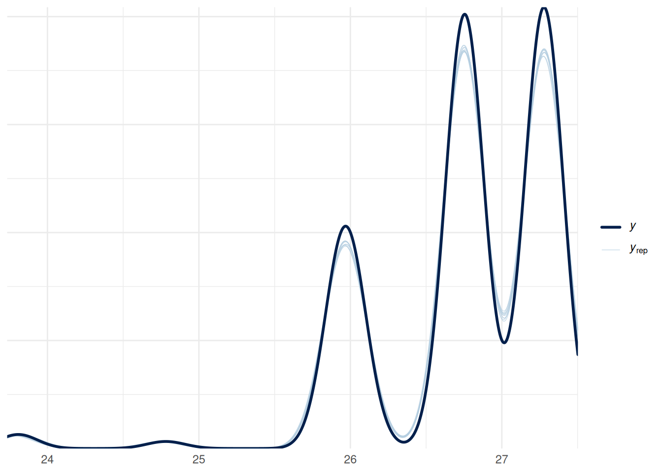
How well did that go? Not so bad, considering all potential sources of error: almost as good as what had been derived from experiments 200 years ago, albeit with larger uncertainty.
g_draws <- fit |>
  as_draws_df(variable = "b_logG_Intercept") |>
  mutate(G = 10^b_logG_Intercept)

g_draws |>
  mean_qi(G) |>
  mutate(rel_uncertainty = (.upper - .lower) / G *100) |>
  print()
# A tibble: 1 × 7
G .lower .upper .width .point .interval rel_uncertainty
<dbl> <dbl> <dbl> <dbl> <chr> <chr> <dbl>
1 6.66682e-11 6.60650e-11 6.72526e-11 0.95 mean qi 1.78133The beauty of Bayesian models is in the posterior distributions, we can look at those:
g_draws |>
  ggplot(aes(x = G)) +
  stat_slab(aes(fill_ramp = after_stat(level)),
                    .width = c(.50, .80, .95, 1),
                    fill = "mediumpurple",
            show.legend = F) +
  geom_vline(xintercept = 6.6743e-11, linetype = 2) +
  annotate("text", x = 6.7e-11, y = 1, label = "What the NIST says") +
  scale_y_continuous(name = NULL, breaks = NULL) +
  labs(caption = "Interval widths: 50%, 80%, 95%, 100%")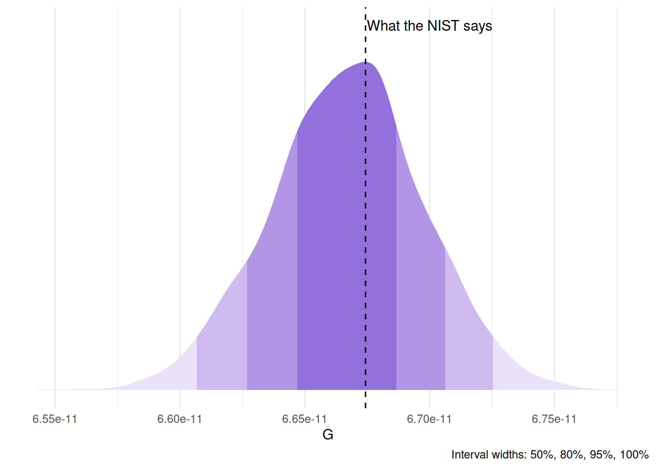
Generate predictions
While this is a fine demonstration of nonlinear brms models, at the beginning I mentioned facing the model with reality. To do this we can take the estimated value of G (with all its posterior distribution) and generate predictions on a separate dataset. In this case, I’ll predict the orbital period of planets around the sun using G, masses, and semi-major axes.
\[T = \sqrt{\frac{4\pi^{2}a^{3}}{G\widehat{M}}}\]
planets <- planets |>
  arrange(sideralOrbit) |>
  mutate(
    englishName = fct(englishName),
    #the mass of the sun in kg
    mass_sun = 1.988475e30,
    M = mass + mass_sun,
    #convert semi-major axis to meters
    a = semimajorAxis * 1000,
    #convert sideral orbit to seconds
    T = sideralOrbit * 24 * 3600,
    #remind the value of pi to the model
    pi = pi)

planets_pred <- planets |>
  expand_grid(G = g_draws$G) |>
  mutate(Tpred = sqrt((4*pi^2*a^3)/(G*M)))

planets_pred |>
  group_by(englishName) |>
  mean_qi(Tpred) |>
  select(!.width:.interval) |>
  left_join(planets |> select(englishName, T)) |>
  mutate(perc_err = (T - Tpred) / T * 100,
         across(Tpred:T, \(x) x |>
                  as.difftime(units = "secs") |>
                  `units<-`("days") |>
                  round(3)),
abs_err = T - Tpred)| englishName | Tpred | .lower | .upper | T | perc_err | abs_err |
|---|---|---|---|---|---|---|
| Mercury | 88.018 days | 87.634 days | 88.418 days | 87.969 days | -0.0552848 | -0.049 days |
| Venus | 224.823 days | 223.843 days | 225.846 days | 224.701 days | -0.0544574 | -0.122 days |
| Earth | 365.459 days | 363.864 days | 367.120 days | 365.256 days | -0.0554693 | -0.203 days |
| Mars | 687.351 days | 684.353 days | 690.476 days | 686.980 days | -0.0539938 | -0.371 days |
| Jupiter | 4335.085 days | 4316.175 days | 4354.796 days | 4332.589 days | -0.0576027 | -2.496 days |
| Saturn | 10761.472 days | 10714.529 days | 10810.402 days | 10759.220 days | -0.0209280 | -2.252 days |
| Uranus | 30719.406 days | 30585.405 days | 30859.081 days | 30685.400 days | -0.1108201 | -34.006 days |
| Neptune | 60259.493 days | 59996.636 days | 60533.482 days | 60189.000 days | -0.1171186 | -70.493 days |
planets_pred |>
  ggplot() +
  stat_pointinterval(aes(y = Tpred)) +
  geom_hline(aes(yintercept = T),
             linetype = 2,
             data = planets |> mutate(T = as.difftime(T, units = "secs"))) +
  facet_wrap(vars(englishName),
             scales = "free") +
  scale_y_time(labels = \(x) str_c(round(x / 3600, 1), " d")) +
  scale_x_discrete() +
  labs(x = NULL,
       y = "Orbital period",
       title = "Predicting orbital periods",
       caption = "Median, 66% and 95% quantile intervals. Dashed line represents official value") +
  theme(plot.title = element_text(hjust = 0.5))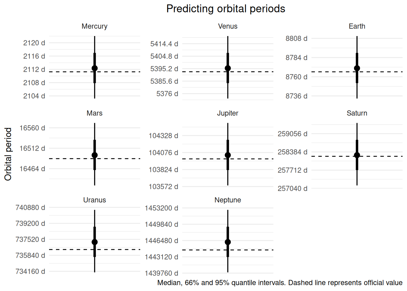
Not too bad! Even with our humble estimation, we can still decently predict the orbit of planets.
References
McElreath, Richard. 2020. Statistical Rethinking: A Bayesian Course with Examples in r and STAN. 2nd ed. Chapman; Hall/CRC. https://doi.org/10.1201/9780429029608.
Meehl, Paul E. 1967. “Theory-Testing in Psychology and Physics: A Methodological Paradox.” Philosophy of Science 34 (2): 103–15. https://doi.org/10.1086/288135.